Why study math? Is it even useful?
Spoiler: use it to solve all your problems and conquer the universe
“Why are we learning this?”
“When am I ever going to use this?”
If you’ve taken a math class, you’ve probably asked those questions. Back when I was a student staring at matrices and derivatives on a whiteboard, it wasn’t obvious what any of it was for. As a teaching assistant, I’ve seen many bright students go through classes without ever being told why the material matters or how it connects to problems they care about. Over time I’ve come to see the answer more clearly through research and building real systems: math gives us a language to describe the world and the tools to understand and shape it.

This post is for anyone who’s taken math classes and felt that disconnect. You might be a student, a researcher in another field, or someone revisiting math with fresh curiosity. If you’re new to these ideas, I’ll try to give enough structure to orient you. If you’re further along, I hope this offers a different angle or sparks new connections.
What follows is the framework I wish I’d had earlier in my career: a way to see how you can use mathematics in your daily life. This covers:
why humans build models of the world in the first place
how different branches of mathematics support this goal,
and how it all connects to problems we face in science, engineering and life.
Let’s dive in.
Why We Build Models
Why do humans build models of the world? Fundamentally, it comes down to our desire to understand, predict, and control the environment around us. Whether it’s the economy, the weather, disease, or a rocket trajectory, we need a simple, precise way to describe reality. A mathematical model is:
A formal representation of the world, defined by variables (system state), parameters (its constants), governing equations (the rules linking them), and constraints that specify how the system behaves.
In summary, we create models because we want to:
Understand how systems work
Predict what might happen next
Control outcomes and make better decisions.
To achieve these aims, we rely on various mathematical frameworks and tools.
The Modeling Toolkit
Each of the following mathematical fields contributes a critical piece of the puzzle. In this post, we’ll walk through them in two parts. The first group provides the language of mathematical modeling; the second shows how we use that language to build and solve real problems.
Part 1: Mathematical Foundations
Linear Algebra: Representing data and relationships
Calculus and Dynamics: Representing change
Probability and Statistics: Representing uncertainty
Part 2: Modeling and Solving
Optimization and Control: Making good decisions
Statistical Learning: Building models from data
Numerical and Computational Methods: Getting computers to solve our problems
Note: This is far from a complete list. The focus of this post is on applied mathematics: how math connects directly to real world applications. Other areas like algebra, discrete math, analysis, information theory, geometry, and topology provide the theoretical foundation that makes this possible. Additionally, this is all just my personal opinion and made up, it’s just a framework I find useful.
Part 1: Mathematical Foundations
We’re going to start with the building blocks that give us the language to even talk about our problems.
Linear Algebra: Represent the World as Mathematical Objects
Linear algebra provides the language to represent the world in mathematical form. It’s how we describe systems and transformations, and how we turn the world into something we can compute and reason about.
The core objects here are vectors and matrices. A vector represents quantities, a set of (usually) numbers with direction and magnitude, and is often used to encode data. A matrix captures relationships: how one set of variables influences another, or how a transformation acts on a vector.
For instance:
An image can be represented as a flattened vector of pixel values
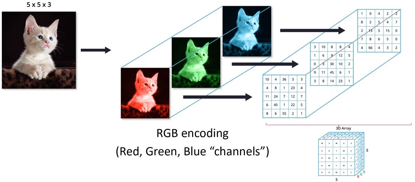
Turn this cat into a vector in our input space (Source: A network can be encoded as a matrix of connections (0 or 1 for edge presence)

A system of equations can be expressed compactly (for matrix A, vector x, constants b) as


Once we’ve expressed the messy, real world in the precise, manipulable form of vector spaces, we can uncover the geometry in data and solve problems. Many tools exist for solving systems of linear equations, like Gaussian elimination and LU decomposition. Operations like eigendecomposition and SVD reveal eigenvalues and singular values, hidden structure that encodes the most important components in a system. These ideas power data compression, facial recognition and Google’s PageRank algorithm.
The world itself isn’t truly linear—true linearity is actually rare. But linear systems are the ones we can understand exactly and compute efficiently. Even nonlinear phenomena are often studied through linear approximations: by zooming in around a point where things look locally linear. This is the core insight of calculus: every smooth curve looks like a line up close. That idea is the bridge to calculus.
Applications: compress images, model networks, simulate physical systems, or analyze relationships in high-dimensional data.
Calculus and Dynamics: Modeling Change
Calculus is the mathematics of change. It’s how we model systems that evolve continuously and describe how things move, grow, or decay. Derivatives measure rates of change while integrals measure accumulation. Together they link local and global behavior and explain how small changes turn into large ones.
When we formalize these relationships for systems by relating a function to its rate of change, we get differential equations. The simplest of these is a dynamical system that relates a system’s current state to its rate of change, like predicting tomorrow’s weather based on how fast it’s cooling now.
This single equation underlies everything from population dynamics to the spread of diseases and planetary motion. The function encodes the governing rule of how the system evolves over time.
These equations let us answer questions like: If we increase this input, how fast does the output respond? Given the current rate of change, where will the system be in the future? This appears in physics (Newton’s laws), engineering (control systems), and biology (epidemic models). Calculus and dynamics, together, give us a framework for understanding motion, feedback, and evolution in the systems around us.
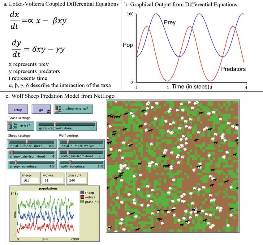
Applications: forecast epidemics, model predator-prey population dynamics, simulate fluid flow, model drone feedback systems, or project long-term climate evolution.
Probability and Statistics: Quantifying Uncertainty
Real life is full of uncertainty. Sensors fail, people behave unpredictably, and data is noisy. Probability and statistics give us the tools to reason in that uncertainty and model uncertainty and variability in the world.
Probability is the language of uncertainty because it gives us a framework to quantify how likely events are. Probability theory defines a mathematical space of possible outcomes, with a distribution assigning each outcome a likelihood. This extends to continuous cases to form the foundation for modeling random processes such as the roll of a die or the fluctuation of stock prices.
Statistics reverses the problem: given data, infer the underlying process.
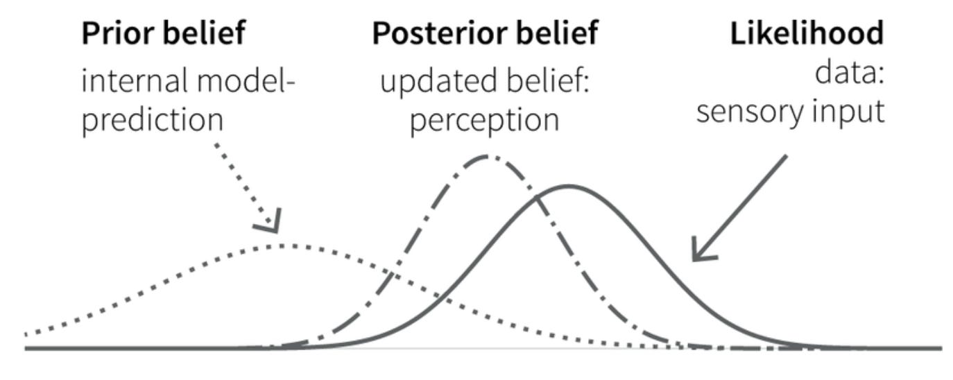
It allows us to build models, estimate parameters and update our beliefs as new information arrives. Bayesian reasoning captures this beautifully:
We start with a prior belief, observe new data, and update accordingly. This is the mathematical version of learning.
Together, probability and statistics enable our models to make predictions with a measure of confidence (for example, a weather forecast might say there’s a 90% chance of rain) and to deal with incomplete information in a principled way. This is also how we reason in everyday life. Checking whether a friend will show up on time, or estimating whether that startup idea will work are all subconsciously doing Bayesian inference: updating beliefs as new evidence comes in.
Applications: weather forecasting, clinical trials, risk estimation, making a lot of money in poker, and any decision where uncertainty is part of the picture.
Part 2: Model and Solve Real-World Problems
Now that we’ve covered how to represent data, change and uncertainty mathematically, we will go over how to model and solve real-world problems.
Statistical Learning: Build models with data
So far, we’ve talked about how math helps us represent the world: how to describe structure with linear algebra, change with calculus, and uncertainty with probability. An interesting question naturally follows: instead of writing down every rule ourselves, what if we let the data teach us the rules?
That’s what statistical learning is, a broad set of techniques for building models that learn from data and improve as more data becomes available. Traditional modeling starts with theory. You write equations that describe how you think the world works, and then test them. Statistical learning flips that around. You start with observations, and use math to infer the structure behind them. It gives us tools like regression, classification, and clustering to find relationships and make predictions without knowing the exact equations in advance.
In that sense, statistical learning is the bridge between modeling and learning: it’s how we turn data into knowledge. Each new datapoint updates our understanding, refining the model to better reflect reality. It’s what allows models to improve the more we observe.
Applications: predict housing prices from features like size and location, detect spam based on language patterns, or group similar behaviors in customer data or biological signals.
Machine Learning: Scaling Statistical Learning
Machine learning is what happens when we take statistical learning and scale it up with more data, more computation, and more flexible models. Machine learning replaces hand-crafted equations with general-purpose systems that can learn almost any relationship, given enough data and compute. What distinguishes ML is that it often avoid making strong a priori assumptions about the form of the model. Instead of assuming a simple formula, ML algorithms learn the non-linear mapping between inputs and outputs from the data itself. This means ML can capture non-linear, emergent patterns that humans might not think to hard-code and cannot infer.
Classical methods like regression, decision trees, random forests, support vector machines and Monte-Carlo do this in transparent, structured ways. They remain the backbone of applied modeling wherever speed and interpretability matter.

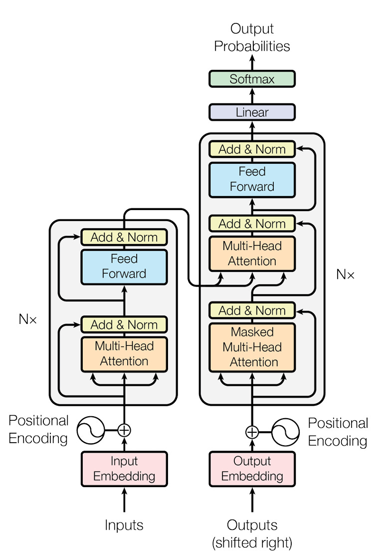
Neural networks take the same idea and make it more flexible. By stacking simple computational layers, they can learn complex, nonlinear relationships directly from data. Deep learning built on this foundation: convolutional networks learned to see, recurrent and LSTM networks learned to remember. Then came transformers, built on attention, able to capture long-range structure in text, images, and sequences. Diffusion models pushed generation further, learning to reverse noise and create realistic images, video, and 3D forms. Reinforcement learning adds a feedback loop, letting models improve through interaction and human guidance (as in RLHF). Combined with self-supervised training, these systems adapt without being explicitly programmed. These architectures now power the “foundation models” behind ChatGPT, AlphaFold, and modern generative AI.
The field is moving fast. New models appear every few months, each expanding what machines can represent or create. As models grow in scale and capability, challenges like interpretability, bias, and control grow with them. But the promise is just as large: machine learning turns data into models that not only describe the world but learn and adapt from it, extending mathematics from analyzing systems to building ones that evolve alongside us.
Applications: prediction (forecast energy demand, recommend treatments, or optimize pricing), learn structure from raw data (protein geometry in AlphaFold), model intelligence itself (neural networks, ChatGPT).
Optimization and Control: Making Good Decisions
Even once we’ve built a model of a system, we still face a critical question: what should we do with it? That’s where optimization comes in, the mathematics of decision-making. It’s how we translate real-world problems and preferences into a formal system we can optimize to make the best possible decision.
Every optimization problem has three parts:
Decision variables: what we can control.
Objective function: what we want to maximize or minimize (e.g. profit, accuracy, efficiency)
Constraints: requirements or preferences (e.g. budgets, limits, physical laws).
With that setup, the problem becomes finding the best possible decision that satisfies the constraints. You’ve likely solved optimization problems without realizing it. When you plan a commute, you’re minimizing travel time subject to road and traffic constraints. A company scheduling workers is maximizing productivity subject to budget and manpower limits. In machine learning, optimization algorithms tune model parameters to minimize prediction error. Every training run is, at its heart, an optimization loop.

Control theory extends this further. It adds feedback, the ability to continuously adjust based on the system’s current state. That’s how autopilot systems keep aircraft stable, or how thermostats regulate temperature. It’s optimization, but done in real time, constantly re-solving the problem as new information comes in.
Optimization and control give us the mathematical framework for making principled, efficient decisions in complex environments. They formalize the intuitive question we all ask: Given what I can control, what’s the best I can do?
Applications: train neural networks (parameter update algorithms like gradient descent), plan robot motion, or optimize complex engineering systems.
Numerical and Computational Methods: Solving Equations with Computers
Once we have models and optimization problems, there’s still one final hurdle: solving them. Most of the time, the real world doesn’t hand us equations that yield neat, exact answers. Numerical and computational methods let us find “good enough” solutions to problems that are too large, nonlinear, or high-dimensional to solve analytically with pen and paper.
We turn to computers to simulate and solve equations approximately and find approximate solutions. This includes techniques from numerical linear algebra, optimization algorithms, and simulation methods. We come full circle here, since linear algebra does most of the heavy lifting in solving systems of equations, computing eigenvalues, and performing matrix factorizations that make large-scale computation possible. The rise of powerful computers has completely changed the landscape: problems once considered impossible, like climate modeling, molecular dynamics, or global optimization, are now routine. Fields like scientific computing and machine learning build on these foundations, using computational methods to turn abstract models into practical tools that can handle real-world complexity. In the end, numerical and computational techniques are the bridge between mathematical models and practical solutions, by using computers to solve our problems.
Applications: Simulate weather systems, run models on supercomputers, render graphics, solve systems of equations of matrices with billions of entries, train deep networks by efficiently crunching data to find optimal parameters.
Conclusion
In our quest to understand, predict, and shape the world, we use a combination of these mathematical tools.
To recap: Linear algebra lets us represent and manipulate structure, calculus models change and dynamics, probability and statistics help us reason under uncertainty; optimization and control guide our decisions, statistical learning builds models that improve with experience, and numerical methods make it all computable.
Together, they form the mathematical modeling toolkit: the set of tools to translate reality into mathematics so we can solve problems. This same toolkit powers breakthroughs across physics, engineering, economics, biology, computer science, neuroscience, climate science, and data science. The details vary by domain, but the core principle remains: master these mathematical tools, and you can model almost anything.
Once you master this toolkit, you’ll be able to invent technologies, make principled decisions, and design systems that actually work. You’ll have to power to build, predict, and shape reality.

Enjoyed reading this, especially the section on Probability Theory
Well written! Looking forward to learning more.